Getting started

Note: For instrument specific guides, please see the IRDB

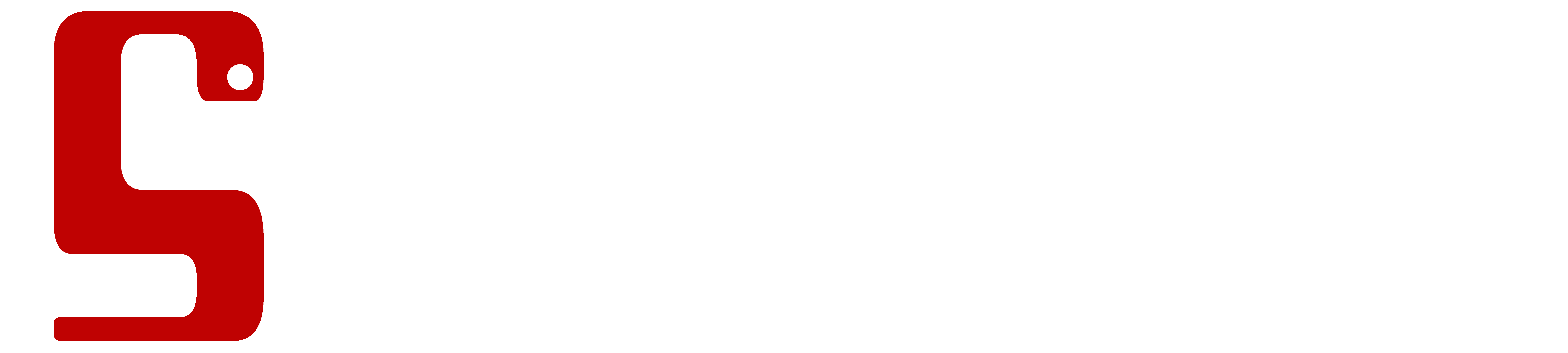
A basic simulation would look something like this:

from matplotlib import pyplot as plt

from scopesim import example_simulation
from scopesim.source.source_templates import star_field

source = star_field(
    n=100, 
    mmax=15,    # [mag]
    mmin=20, 
    width=200,  # [arcsec]
)

simulation = example_simulation()
hdulist = simulation(source, dit=60, ndit=10)  # dit and ndit in seconds

plt.figure(figsize=(10, 8))
plt.imshow(hdulist[1].data, origin="lower", norm="log")
plt.colorbar()

astar.scopesim.detector.detector_manager - Extracting from 1 detectors...

<matplotlib.colorbar.Colorbar at 0x7f85a6f04a50>

Code breakdown

Let’s break this down a bit.

There are three major components of any simulation workflow:

1. the target description,

2. the telescope/instrument model, and

3. the observation.

For the target description we are using the ScopeSim internal template functions from scopesim.source.source_templates, however many more dedicated science related templates are available in the external python package ScopeSim-Templates

Here we create a field of 100 A0V stars with Vega magnitudes between V=15 and V=20 within a box of 200 arcsec:

source = star_field(
    n=100, 
    mmax=15,    # [mag]
    mmin=20, 
    width=200,  # [arcsec]
)

Next we load the sample optical train object from ScopeSim.

Normally we will want to use an actual instrument. Dedicated documentation for real telescope+instrument systems can be found in the documentation sections of the individual instruments in the Instrument Reference Database (IRDB) documentation

For real instruments loading the optical system generally follows a different pattern:

from scopesim import Simulation
simulation = Simulation("instrument_name", mode="instrument_mode")

or, for instruments with combination modes (e.g. MICADO):

simulation = Simulation("instrument_name", mode=["mode_1", "mode_2"])

Once we have loaded the instrument, we can set the observation parameters by accessing the internal settings dictionary:

simulation = example_simulation(mode="imaging")
simulation.settings["!OBS.dit"] = 60   # [s]
simulation.settings["!OBS.ndit"] = 10

Finally we observe the target source and readout the detectors, which can be done by simly calling the simulation instance.

What is returned (hdulist) is an astropy.fits.HDUList object which can be saved to disk in the standard way, or manipulated in a python session.

simulation(source)

astar.scopesim.detector.detector_manager - Extracting from 1 detectors...

[<astropy.io.fits.hdu.image.PrimaryHDU object at 0x7f85a65043d0>, <astropy.io.fits.hdu.image.ImageHDU object at 0x7f85a63296d0>]

Tips and tricks

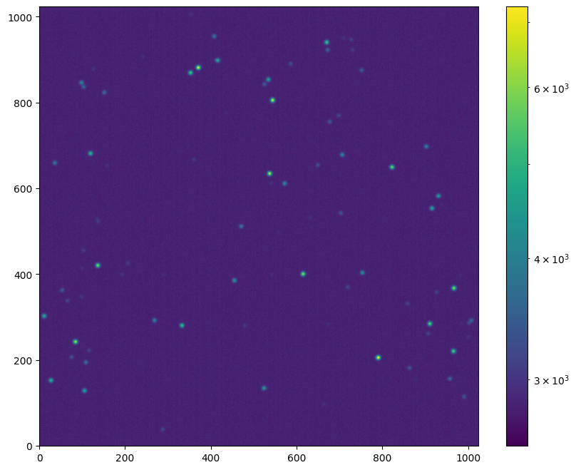
Focal plane images

Intermediate frames of the focal plane image without the noise proerties can be accessed by looking inside the optical train object and accessing the first image plane:

noiseless_image = simulation.optical_train.image_planes[0].data
plt.figure(figsize=(10, 8))
plt.imshow(noiseless_image, origin="lower")
plt.colorbar()

<matplotlib.colorbar.Colorbar at 0x7f85a6332510>

Turning optical effects on or off

All effects modelled by the optical train can be listed with the .effects attribute:

simulation.optical_train.effects

Table length=19

element	name	class	included
str16	str22	str29	bool
basic_atmosphere	atmospheric_radiometry	AtmosphericTERCurve	True
basic_telescope	psf	SeeingPSF	True
basic_telescope	telescope_reflection	TERCurve	True
basic_instrument	static_surfaces	SurfaceList	True
basic_instrument	filter_wheel : [J]	FilterWheel	True
basic_instrument	slit_wheel : [narrow]	SlitWheel	False
basic_instrument	image_slicer	ApertureList	False
basic_detector	detector_window	DetectorWindow	True
basic_detector	detector_3d	DetectorList3D	False
basic_detector	qe_curve	QuantumEfficiencyCurve	True
basic_detector	exposure_integration	ExposureIntegration	True
basic_detector	dark_current	DarkCurrent	True
basic_detector	shot_noise	ShotNoise	True
basic_detector	detector_linearity	LinearityCurve	True
basic_detector	readout_noise	PoorMansHxRGReadoutNoise	True
basic_detector	source_fits_keywords	SourceDescriptionFitsKeywords	True
basic_detector	effects_fits_keywords	EffectsMetaKeywords	True
basic_detector	config_fits_keywords	SimulationConfigFitsKeywords	True
basic_detector	extra_fits_keywords	ExtraFitsKeywords	True

These can be turned on or off by using their name and the .include attribute:

simulation.optical_train["detector_linearity"].include = False

Listing available modes and filters

The list of observing modes can be found by using the .modes attribute of the commands objects:

simulation.settings.modes

imaging: Basic NIR imager, status=development
spectroscopy: Basic three-trace long-slit spectrograph, status=development
ifu: Basic three-trace integral-field-unit spectrograph, status=development
simple_ifu: For testing the virtual 3D Detector with direct cube output, status=development
mock_concept_mode: Dummy mode to test concept status., status=concept
mock_experimental_mode: Dummy mode to test experimental status., status=experimental
mock_deprecated_mode: Dummy mode to test deprecated status without message., status=deprecated
mock_deprecated_mode_msg: Dummy mode to test deprecated status with message., status=deprecated

The names of included filters can be found in the filter effect. Use the name of the filter object from the table above to list these:

simulation.optical_train["filter_wheel"].filters

{'BrGamma': FilterCurve: "BrGamma",
 'CH4': FilterCurve: "CH4",
 'J': FilterCurve: "J",
 'H': FilterCurve: "H",
 'Ks': FilterCurve: "Ks",
 'open': FilterCurve: "open"}

Setting observation sequence

Although this could be different for some instruments, most instruments use the exptime = ndit * dit format. nditand dit are generally accessible in the top level !OBS dictionary of the command object in the optical train.

simulation.settings["!OBS.dit"] = 60   # [s]
simulation.settings["!OBS.ndit"] = 10

Listing and changing simulation parameters

The command dictionary inside the optical system contains all the necessary paramters.

simulation.settings

CurrObs

❗OBS

• exptime: None
• dit: 60
• ndit: 10

CurrSys

❗OBS

• instrument: basic_instrument
• psf_fwhm: 1.5
• modes: ['imaging']
• dit: 60
• ndit: 10
• slit_name: narrow
• wavelen: 2.1
• include_slit: False
• include_slicer: False
• include_det_window: True
• include_det_3d: False
• filter_name: J

❗ATMO

• background:
  • filter_name: J
  • value: 16.6
  • unit: mag

❗TEL

• telescope: Basic Telescope
• temperature: 0
• area: 0.19634954084936207 m2
• etendue: 0.007853981633974483 arcsec2 m2

❗INST

• temperature: -190
• pixel_scale: 0.2
• plate_scale: 20

❗DET

• image_plane_id: 0
• temperature: -230
• dit: !OBS.dit
• ndit: !OBS.ndit
• width: 1024
• height: 1024
• x: 0
• y: 0

SystemDict

❗SIM

• spectral:
  • wave_min: 0.3
  • wave_mid: 2.2
  • wave_max: 20
  • wave_unit: um
  • spectral_bin_width: 0.0001
  • spectral_resolution: 5000
  • minimum_throughput: 1e-06
  • minimum_pixel_flux: 1
• sub_pixel:
  • flag: False
  • fraction: 1
• random:
  • seed: None
• computing:
  • chunk_size: 2048
  • max_segment_size: 16777217
  • oversampling: 1
  • spline_order: 1
  • flux_accuracy: 0.001
  • preload_field_of_views: False
  • nan_fill_value: 0.0
• file:
  • example_data:
    • suburl: example_data
    • hash_file: example_data_registry.txt
  • psfs:
    • suburl: psfs
    • hash_file: psfs_registry.txt
  • atmo:
    • suburl: atmo
    • hash_file: atmo_registry.txt
  • local_packages_path: /home/docs/checkouts/readthedocs.org/user_builds/scopesim/checkouts/stable/scopesim/tests/mocks
  • server_base_url: https://scopesim.univie.ac.at/InstPkgSvr/
  • retries: 3
  • use_cached_downloads: False
  • search_path: ['./inst_pkgs/', './']
  • error_on_missing_file: False
• reports:
  • ip_tracking: False
  • verbose: False
  • rst_path: ./reports/rst/
  • latex_path: ./reports/latex/
  • image_path: ./reports/images/
  • image_format: png
  • preamble_file: None
• tests:
  • run_integration_tests: True
  • run_skycalc_ter_tests: True

❗OBS

❗TEL

• etendue: 0
• area: 0

❗INST

• pixel_scale: 0
• plate_scale: 0
• decouple_detector_from_sky_headers: False

The command object is a series of nested dictionaries that can be accessed using the !-string format:

simulation.settings["!<alias>.<param>"]
simulation.settings["!<alias>.<sub_dict>.<param>"]

For example, setting the atmospheric background level is achieved thusly:

simulation.settings["!ATMO.background.filter_name"] = "K"
simulation.settings["!ATMO.background.value"] = 13.6

The updated parameters (and the previous defaults) can be viewed by querying the "!ATMO" section. Values in higher levels always override defaults in lower levels.

simulation.settings["!ATMO"]

[0] mapping

• background:
  • filter_name: K
  • value: 13.6

[1] mapping

• background:
  • filter_name: J
  • value: 16.6
  • unit: mag

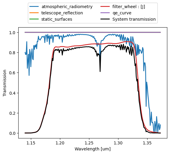
Inspecting the system transmission

The total system transmission and the contribution from the individual elements in the optical train can be visualised as follows:

simulation.optical_train.optics_manager.system_transmission(plot=True);

More information

For more information on how to use ScopeSim be see:

• Use Examples

• Instrument Specific Documentation

• Effect data formats

• Setting up a custom instrument

Contact

• For bugs, please add an issue to the github repo

• For enquiries on implementing your own instrument package, please drop us a line at astar.astro@univie.ac.at or kieran.leschinski@univie.ac.at