1: A quick use case for MICADO at the ELT#
A brief introduction into using ScopeSim to observe a cluster in the LMC#
First set up all relevant imports:
import matplotlib.pyplot as plt

from scopesim import Simulation
from scopesim_templates.stellar.clusters import cluster
Now, create a star cluster as the source using the scopesim_templates package. You can ignore the output that is sometimes printed. The seed argument is used to control the random number generation that creates the stars in the cluster. If this number is kept the same, the output will be consistent with each run, otherwise the position and brightness of the stars is randomised every time.
source = cluster(
    mass=1000,        # Msun
    distance=50000,   # parsec
    core_radius=0.3,  # parsec
    seed=9002,        # random number seed
)
imf - sample_imf: Setting maximum allowed mass to 1000
imf - sample_imf: Loop 0 added 1.26e+03 Msun to previous total of 0.00e+00 Msun
Next, create the MICADO optical system model with the new simplified Simulation interface. Observe the cluster Source object simply by calling the simulation instance, which returns the resulting FITS HDUL. This may take a few moments on slower machines.
The resulting FITS file can either be returned as an astropy.fits.HDUList object, which can be saved to disk using the writeto method.
simulation = Simulation("MICADO", ["SCAO", "IMG_4mas"])
hdul = simulation(source)
# hdul.writeto("TEST.fits")
httpxyz - HTTP Request: POST https://etimecalret-002.eso.org/observing/etc/api/skycalc "HTTP/1.1 200 OK"
httpxyz - HTTP Request: GET https://etimecalret-002.eso.org/observing/etc/api/rmtmp?d=e8106c23-df5a-48cx-8d76-73d062aa1450 "HTTP/1.1 200 OK"
astar.scopesim.detector.detector_manager - Extracting from 1 detectors...
astar.scopesim.effects.electronic.electrons - Applying gain 1
astar.scopesim.effects.fits_headers - WARNING: #exposure_action.include not found
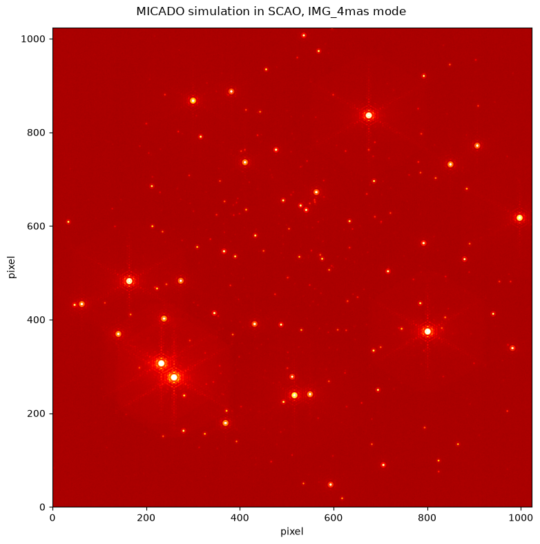
Plot the results of the simulation. The fig_kwargs are passed to matplotlib’s figure creation.
simulation.plot(norm="log", vmin=3e3, vmax=3e4, cmap="hot",
                fig_kwargs={"figsize": (8, 8), "layout": "tight"})
(<Figure size 800x800 with 1 Axes>, [<Axes: xlabel='pixel', ylabel='pixel'>])