Creating Custom Effects

ScopeSim’s built-in effects cover the most common physical phenomena in optical systems, but you may need to model instrument-specific behaviour that isn’t provided out of the box. Creating a custom Effect subclass lets you inject arbitrary transformations into the simulation pipeline.

For a worked example that creates a PointSourceJitter effect and adds it to a full MICADO simulation, see the Custom Effects Example Notebook. This page focuses on a complementary example – a non-symmetric vignetting flat field applied at the image plane level.

Anatomy of an Effect Subclass

Every custom effect needs three things:

1. z_order – a class variable (tuple of ints) that tells ScopeSim when in the pipeline to apply the effect.

2. __init__ – calls super().__init__() and sets default parameters in self.meta.

3. apply_to(self, obj) – the method that does the work. It receives an object, optionally modifies it, and must return it.

The apply_to method should use isinstance checks to determine whether to act on the given object. During a simulation run, ScopeSim passes different object types at different stages – your effect will only modify the types it knows how to handle, and pass everything else through unchanged.

Choosing the Right Z-Order

The z_order determines which pipeline stage your effect participates in, and therefore what type of object it receives:

Z-Order Range	Object Type	Use When…
500–599	Source	Modifying the original light distribution (e.g., spectral shifts, flux scaling)
600–699	FieldOfView	Modifying per-wavelength spatial cutouts (e.g., PSF convolution, dispersion)
700–799	ImagePlane	Modifying the wavelength-integrated focal plane image (e.g., vignetting, flat fields)
800–899	Detector	Modifying the detector readout (e.g., noise, dark current, gain variations)

An effect can have multiple z_order values to participate in both a setup stage and an application stage. For a simple custom effect, a single value is usually sufficient.

Example: Non-Symmetric Vignetting Flat Field

This example creates an effect that applies a spatially-varying throughput pattern to the image plane, simulating optical vignetting that is not radially symmetric – for instance, caused by an off-axis obstruction or asymmetric optics.

The vignetting is modelled as an elliptical Gaussian decay with configurable center offset, semi-axes, rotation angle, and throughput range.

Defining the effect class

import numpy as np
from scopesim.effects import Effect
from scopesim.optics.image_plane import ImagePlane


class NonSymmetricVignetting(Effect):
    """Apply a non-symmetric vignetting pattern to the image plane."""

    z_order = (710,)

    def __init__(self, **kwargs):
        super().__init__(**kwargs)
        params = {
            "x_center_offset": 0.1,    # fractional offset from image center
            "y_center_offset": -0.05,
            "sigma_x": 0.8,            # fractional semi-axis (1.0 = full frame)
            "sigma_y": 0.6,
            "rotation_deg": 15.0,       # rotation angle of the vignetting ellipse
            "max_throughput": 1.0,
            "min_throughput": 0.3,
        }
        for key, val in params.items():
            self.meta.setdefault(key, val)
        self.meta.update(kwargs)

    def _make_vignetting_map(self, shape):
        """Generate a 2D vignetting map for a given image shape."""
        ny, nx = shape
        y, x = np.mgrid[:ny, :nx]

        # Normalise pixel coordinates to [-1, 1] and apply center offset
        x_norm = 2.0 * x / nx - 1.0 - self.meta["x_center_offset"]
        y_norm = 2.0 * y / ny - 1.0 - self.meta["y_center_offset"]

        # Rotate coordinate frame
        angle = np.deg2rad(self.meta["rotation_deg"])
        cos_a, sin_a = np.cos(angle), np.sin(angle)
        x_rot = x_norm * cos_a + y_norm * sin_a
        y_rot = -x_norm * sin_a + y_norm * cos_a

        # Elliptical Gaussian falloff
        r2 = (x_rot / self.meta["sigma_x"]) ** 2 + \
             (y_rot / self.meta["sigma_y"]) ** 2
        t_min = self.meta["min_throughput"]
        t_max = self.meta["max_throughput"]
        vmap = t_min + (t_max - t_min) * np.exp(-0.5 * r2)

        return np.clip(vmap, t_min, t_max)

    def apply_to(self, obj, **kwargs):
        if isinstance(obj, ImagePlane):
            vignetting = self._make_vignetting_map(obj.hdu.data.shape)
            obj.hdu.data *= vignetting
        return obj

Setting up the simulation

import scopesim as sim
from scopesim.source.source_templates import star_field

# Load the example optical train and create a star field source
opt = sim.load_example_optical_train()
src = star_field(n=50, mmin=15, mmax=20, width=200)

# Create and add the vignetting effect
vig = NonSymmetricVignetting(name="asymmetric_vignetting")
opt.optics_manager.add_effect(vig)

opt.effects

Table length=20

element	name	class	included
str16	str22	str29	bool
basic_atmosphere	atmospheric_radiometry	AtmosphericTERCurve	True
basic_atmosphere	asymmetric_vignetting	NonSymmetricVignetting	True
basic_telescope	psf	SeeingPSF	True
basic_telescope	telescope_reflection	TERCurve	True
basic_instrument	static_surfaces	SurfaceList	True
basic_instrument	filter_wheel : [J]	FilterWheel	True
basic_instrument	slit_wheel : [narrow]	SlitWheel	False
basic_instrument	image_slicer	ApertureList	False
basic_detector	detector_window	DetectorWindow	True
basic_detector	detector_3d	DetectorList3D	False
basic_detector	qe_curve	QuantumEfficiencyCurve	True
basic_detector	exposure_integration	ExposureIntegration	True
basic_detector	dark_current	DarkCurrent	True
basic_detector	shot_noise	ShotNoise	True
basic_detector	detector_linearity	LinearityCurve	True
basic_detector	readout_noise	PoorMansHxRGReadoutNoise	True
basic_detector	source_fits_keywords	SourceDescriptionFitsKeywords	True
basic_detector	effects_fits_keywords	EffectsMetaKeywords	True
basic_detector	config_fits_keywords	SimulationConfigFitsKeywords	True
basic_detector	extra_fits_keywords	ExtraFitsKeywords	True

Observing and visualising

import matplotlib.pyplot as plt

opt.observe(src, update=True)

fig, axes = plt.subplots(1, 2, figsize=(14, 5))

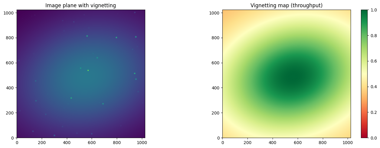
# Show the vignetted image
axes[0].imshow(opt.image_planes[0].data, origin="lower")
axes[0].set_title("Image plane with vignetting")

# Show the vignetting map itself
vmap = vig._make_vignetting_map(opt.image_planes[0].data.shape)
im = axes[1].imshow(vmap, origin="lower", cmap="RdYlGn", vmin=0, vmax=1)
axes[1].set_title("Vignetting map (throughput)")
fig.colorbar(im, ax=axes[1])

plt.tight_layout()
plt.show()

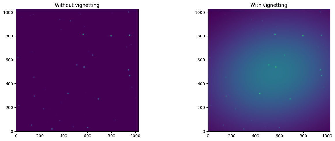
Comparing with and without vignetting

# Observe without vignetting
vig.include = False
opt.observe(src, update=True)
no_vig_data = opt.image_planes[0].data.copy()

# Observe with vignetting
vig.include = True
opt.observe(src, update=True)
vig_data = opt.image_planes[0].data.copy()

fig, axes = plt.subplots(1, 2, figsize=(14, 5))
axes[0].imshow(no_vig_data, origin="lower")
axes[0].set_title("Without vignetting")
axes[1].imshow(vig_data, origin="lower")
axes[1].set_title("With vignetting")
plt.tight_layout()
plt.show()

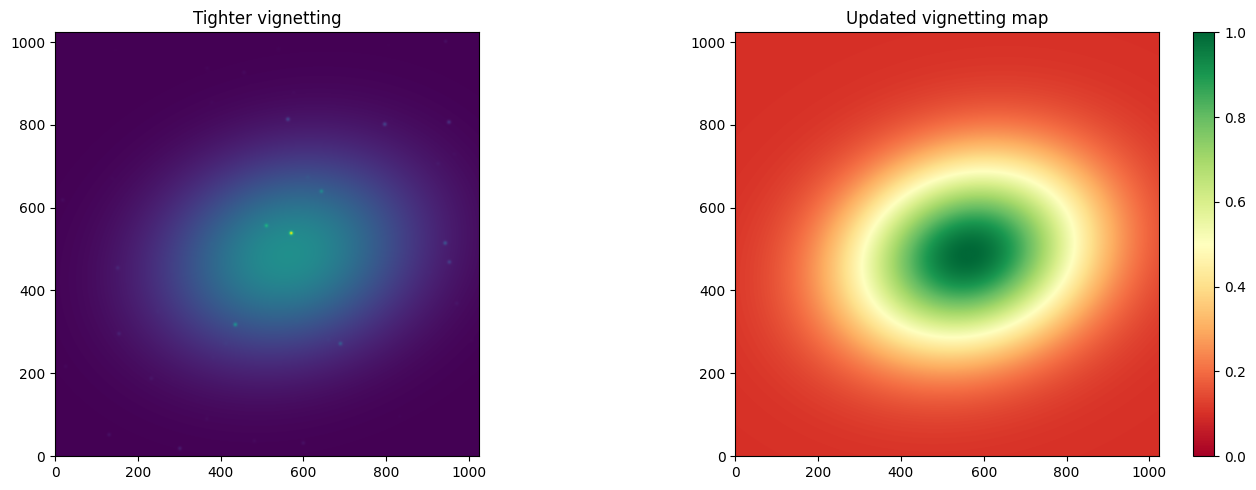
Modifying Parameters at Runtime

Effect parameters live in the .meta dictionary and can be changed between observations:

# Make the vignetting more extreme
opt["asymmetric_vignetting"].meta["sigma_x"] = 0.4
opt["asymmetric_vignetting"].meta["sigma_y"] = 0.3
opt["asymmetric_vignetting"].meta["min_throughput"] = 0.1

opt.observe(src, update=True)

fig, axes = plt.subplots(1, 2, figsize=(14, 5))
axes[0].imshow(opt.image_planes[0].data, origin="lower")
axes[0].set_title("Tighter vignetting")

vmap = vig._make_vignetting_map(opt.image_planes[0].data.shape)
im = axes[1].imshow(vmap, origin="lower", cmap="RdYlGn", vmin=0, vmax=1)
axes[1].set_title("Updated vignetting map")
fig.colorbar(im, ax=axes[1])
plt.tight_layout()
plt.show()

Tips for Writing Robust Effects

• Always return obj from apply_to, even when your isinstance check doesn’t match. ScopeSim passes many object types through the same list of effects – returning None will break the pipeline.

• Use isinstance guards to decide whether to act. Your apply_to will be called with Source, FieldOfView, ImagePlane, and Detector objects at different stages.

• Choose the right pipeline stage carefully:

  • FieldOfView (z=600–699): your effect is applied per wavelength bin and per spatial chunk – appropriate for wavelength-dependent effects.

  • ImagePlane (z=700–799): your effect sees the wavelength-integrated focal plane image – appropriate for achromatic spatial effects like vignetting.

  • Detector (z=800–899): your effect sees the detector readout after extraction – appropriate for electronic effects like noise.

• Look at built-in effects for patterns. For example, PixelResponseNonUniformity in scopesim/effects/electronic/noise.py is a simple multiplicative detector-level effect. SeeingPSF in scopesim/effects/psfs/analytical.py shows how to build a convolution kernel.

• Use from_currsys for parameters that should be resolvable as bang strings (!OBS.some_param):

  from scopesim.utils import from_currsys
  value = from_currsys(self.meta["my_param"], self.cmds)
  

Adding Custom Effects to the Optical Train

Custom effects are added programmatically using optics_manager.add_effect():

my_effect = MyCustomEffect(name="my_effect", some_param=42)
opt.optics_manager.add_effect(my_effect)

After adding an effect, pass update=True to opt.observe() so the optical train rebuilds its internal structures to include the new effect.

Note that YAML-based instrument packages resolve effect class names from the scopesim.effects namespace. Custom effect classes from third-party packages currently need to be added programmatically as shown above.

Sharing Your Custom Effect

Once you’ve written and tested a custom effect, there are several ways to make it available for use – either for yourself or for the wider community.

Option 1: Add it directly to the ScopeSim effects module (local)

If you want your effect to be available via YAML instrument packages (i.e., referenced by class name in a YAML file), the simplest approach is to place your Python file inside the scopesim/effects/ directory of your local ScopeSim installation and import it in scopesim/effects/__init__.py.

For example, if you save your effect class in scopesim/effects/my_vignetting.py:

# scopesim/effects/my_vignetting.py
from .effects import Effect

class NonSymmetricVignetting(Effect):
    ...

Then add the import to scopesim/effects/__init__.py:

from .my_vignetting import *

After this, the class name NonSymmetricVignetting can be used directly in YAML configuration files:

effects:
  - name: vignetting
    class: NonSymmetricVignetting
    kwargs:
      sigma_x: 0.8
      sigma_y: 0.6

Note that this modifies your local ScopeSim installation and will be overwritten when you upgrade the package. For a more permanent solution, consider contributing it upstream (Option 3).

Option 2: Keep it in your own script or package

For effects that are specific to your analysis, you can keep the effect class in your own Python script or package and add it programmatically at runtime as shown above. This is the simplest approach and doesn’t require modifying ScopeSim itself.

Option 3: Contribute it to ScopeSim

If your effect is general-purpose and would be useful to other users, we welcome contributions! You can:

• Open an issue on the ScopeSim GitHub repository describing your effect and sharing the code. The ScopeSim team can help integrate it into the package.

• Submit a pull request with your effect class added to the scopesim/effects/ module, including the import in __init__.py and ideally a test in scopesim/tests/. See the existing effects for examples of the expected code style and structure.

See Also

• Effects Overview – reference for all built-in effect types and the simulation pipeline

• Custom Effects Example Notebook – a worked example with PointSourceJitter and MICADO

• The auto-generated API Reference for scopesim.effects.Effect