2: Observing the same object with multiple telescopes

A brief introduction into using ScopeSim to observe a cluster in the LMC using the 39m ELT and the 1.5m LFOA

First set up all relevant imports:

import matplotlib.pyplot as plt

from scopesim import Simulation
from scopesim_templates.stellar.clusters import cluster

Create a star cluster Source object

Now, create a star cluster using the scopesim_templates package. You can ignore the output that is sometimes printed. The seed argument is used to control the random number generation that creates the stars in the cluster. If this number is kept the same, the output will be consistent with each run, otherwise the position and brightness of the stars is randomised every time.

source = cluster(
    mass=10000,       # Msun
    distance=50000,   # parsec
    core_radius=2.1,  # parsec
    seed=9001,        # random number seed
)

imf - sample_imf: Setting maximum allowed mass to 10000
imf - sample_imf: Loop 0 added 1.01e+04 Msun to previous total of 0.00e+00 Msun

Observe the source

Observe with the 1.5m telescope at the LFOA

lfoa = Simulation("LFOA")
data_lfoa = lfoa(source, dit=10, ndit=360)[1].data

astar.scopesim.commands.user_commands - The selected instrument package is still in experimental stage, results may not be representative of physical instrument, use with care.
astar.scopesim.detector.detector_manager - Extracting from 1 detectors...
astar.scopesim.optics.optical_train - ERROR: Header update failed, data will be saved with incomplete header. See stack trace for details.
Traceback (most recent call last):
  File "/home/docs/checkouts/readthedocs.org/user_builds/scopesim/checkouts/docs-effects-documentation/scopesim/optics/optical_train.py", line 475, in readout
    hdul = self.write_header(hdul)
           ^^^^^^^^^^^^^^^^^^^^^^^
  File "/home/docs/checkouts/readthedocs.org/user_builds/scopesim/checkouts/docs-effects-documentation/scopesim/optics/optical_train.py", line 504, in write_header
    pheader["INSTRUME"] = from_currsys("!OBS.instrument", self.cmds)
                          ^^^^^^^^^^^^^^^^^^^^^^^^^^^^^^^^^^^^^^^^^^
  File "/home/docs/checkouts/readthedocs.org/user_builds/scopesim/checkouts/docs-effects-documentation/scopesim/utils.py", line 625, in from_currsys
    raise ValueError(f"{item} was not found in rc.__currsys__")
ValueError: !OBS.instrument was not found in rc.__currsys__

Observe the same Source with MICADO at the ELT

micado = Simulation("MICADO")
# Use the central detector of the full MICADO array
micado.optical_train["detector_window"].include = False
micado.optical_train["full_detector_array"].include = True
micado.optical_train["full_detector_array"].meta["active_detectors"] = [5]

data_micado = micado(source, dit=10, ndit=360)[1].data

astar.scopesim.detector.detector_manager - Extracting from 1 detectors...
astar.scopesim.effects.ter_curves - Applying border [0, 0, 0, 0]
astar.scopesim.effects.electronic.electrons - Applying gain 1
astar.scopesim.effects.electronic.electrons - Applying digitization to dtype float32.
astar.scopesim.effects.fits_headers - WARNING: #exposure_action.include not found

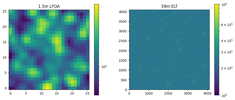
Plot up the results

LFOA has a larger field of view and a lower resolution than MICADO, so while LFOA shows the whole cluster, MICADO only shows the center.

fig, (ax1, ax2) = plt.subplots(1, 2, figsize=(12, 5))

img_lfoa = ax1.imshow(data_lfoa, norm="log", origin="lower")
fig.colorbar(img_lfoa, ax=ax1)
ax1.set_title("1.5m LFOA")

img_micado = ax2.imshow(data_micado, norm="log", vmin=1e5, vmax=1e6, origin="lower")
fig.colorbar(img_micado, ax=ax2)
ax2.set_title("39m ELT")

Text(0.5, 1.0, '39m ELT')

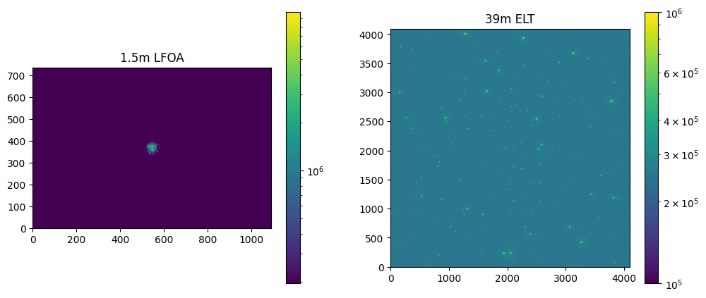
Zoom in the LFOA observation

We can use the pixel scale of LFOA and MICADO to cut out the exact piece of the LFOA observation that corresponds to the MICADO one.

pixel_scale_lfoa = lfoa.settings["!INST.pixel_scale"]
pixel_scale_micado = micado.settings["!INST.pixel_scale"]
scale_factor = pixel_scale_lfoa / pixel_scale_micado

size_lfoa_x = data_micado.shape[0] / scale_factor /2
size_lfoa_y = data_micado.shape[1] / scale_factor /2

xcen_lfoa = data_lfoa.shape[0] / 2
ycen_lfoa = data_lfoa.shape[1] / 2

x_low = round(xcen_lfoa - size_lfoa_x / 2)
x_high = round(xcen_lfoa + size_lfoa_x / 2)
y_low = round(ycen_lfoa - size_lfoa_y / 2)
y_high = round(ycen_lfoa + size_lfoa_y / 2)

fig, (ax1, ax2) = plt.subplots(1, 2, figsize=(12, 5))

img_lfoa = ax1.imshow(data_lfoa[x_low:x_high, y_low:y_high], norm="log", origin="lower")
fig.colorbar(img_lfoa, ax=ax1)
ax1.set_title("1.5m LFOA")

img_micado = ax2.imshow(data_micado, norm="log", vmin=1e5, vmax=1e6, origin="lower")
fig.colorbar(img_micado, ax=ax2)
ax2.set_title("39m ELT")

# fig.savefig("withfullarray.png")

Text(0.5, 1.0, '39m ELT')